Mad Chemiker

本稿は TeX & LaTeX Advent Calendar 2017 の15日目の記事です。
14日目は p_typo さん でした。16日目は keisuke495500 さん です。

本稿ではタイトルの通り、図に注釈等を入れる方法について紹介します。なお確認は pdfLaTeX でのみ行っています。

プリアンブルはこんな感じです。必要なライブラリー等はそれぞれに記載していますが、もしかしたら間違っているかもしれません。その場合はこのプリアンブルで試してみて下さい。

\documentclass{article}
\usepackage[a4paper,height=.8\paperheight,width=.75\paperwidth]{geometry}
\usepackage{tikz}
\usetikzlibrary{calc}
\usetikzlibrary{shapes.callouts}
\usetikzlibrary{spy}
\usetikzlibrary{positioning}
\usepackage{amsmath}
\usepackage[wby]{callouts}
\usepackage{gnuplot-lua-tikz}
\usepackage{tikzducks}

キホン

すでにご存知のことと思いますが \LaTeX で画像ファイルを取り込む代表的な方法は \includegraphics を使用することです。

さて、この図の中に補足情報等を書き入れたい、という場合は以下のようにすることができます。

% duck-grid-noscope.tex
\begin{tikzpicture}
  \node[anchor=south west,inner sep=0] (duck) at (0,0) {%
    \includegraphics[width=0.75\textwidth]{640px-Duck0001.jpg}%
  };
  % 補助
  \draw[help lines] (0,0) grid (12,8);
  \foreach \x in {0,1,...,12} { \node [anchor=north] at (\x,0) {\x}; }
  \foreach \y in {0,1,...,8} { \node [anchor=east]  at (0,\y) {\y}; }
\end{tikzpicture}

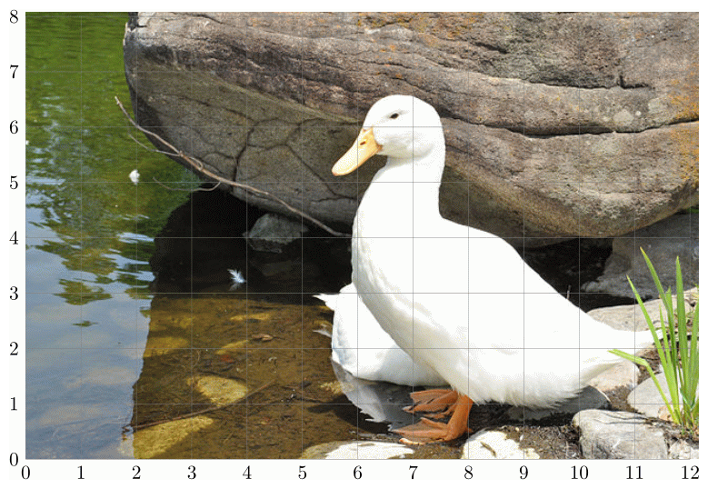
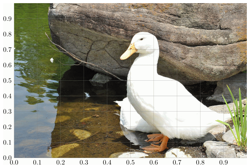
つまり単に node として \includegraphics した図を入れれば OK です (この他に overpic.sty を使う方法もありますが、本稿では扱いません)。あとは座標を指定して \node なり \draw なりをちまちま書いていくだけです。が、この座標系だと位置指定が結構大変です。これを (0,0) – (1,1) になるようにすると、若干ラクになる (場合がある) かもしれません。ポイントとしては、このノード (= 画像) に名前 (アンカー, ここでは (duck)) を付けておき、これをもとに scope で座標系を定めることです。

% duck-onlygrid.tex
\begin{tikzpicture}
  \node[anchor=south west,inner sep=0] (duck) at (0,0) {%
    \includegraphics[width=0.75\textwidth]{640px-Duck0001.jpg}%
  };
  \begin{scope}[x={(duck.south east)},y={(duck.north west)}]
    % 補助
    \draw[help lines,xstep=.1,ystep=.1] (0,0) grid (1,1);
    \foreach \x in {0,1,...,9} { \node [anchor=north] at (\x/10,0) {0.\x}; }
    \foreach \y in {0,1,...,9} { \node [anchor=east]  at (0,\y/10) {0.\y}; }
  \end{scope}
\end{tikzpicture}   

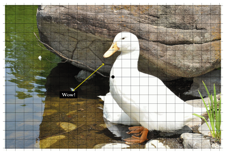
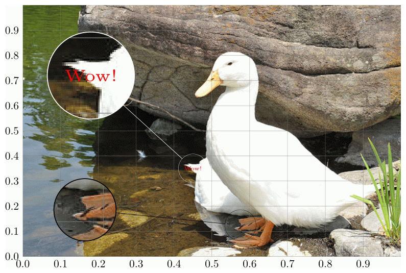
あとは、この補助線を参考に、必要な情報を書き入れていけばなかなか良い感じに仕上ります。

% duck-node.tex
\begin{tikzpicture}
  \node[anchor=south west,inner sep=0] (duck) at (0,0) {%
    \includegraphics[width=0.75\textwidth]{640px-Duck0001.jpg}%
  };
  \begin{scope}[x={(duck.south east)},y={(duck.north west)}]
    % 補助
    \draw[help lines,xstep=.1,ystep=.1] (0,0) grid (1,1);
    \foreach \x in {0,1,...,9} { \node [anchor=north] at (\x/10,0) {0.\x}; }
    \foreach \y in {0,1,...,9} { \node [anchor=east]  at (0,\y/10) {0.\y}; }

    % 注釈
    \node[white, left] at (0.3,0.6) { \bf Wow! };
    \draw[->, white, line width = 2pt] (0.3,0.6) -- (0.43,0.63);
  \end{scope}
\end{tikzpicture}   

位置調整が終わったら補助線を消しておきましょう。

この例では、右下を (0,0)、左上を (1,1) とする座標系を設定していますが、場合によっては変更した方が便利な場合もあります。その場合は calc ライブラリーを使うといい感じにできます。

% sudoku.tex
% \usetikzlibrary{calc}

\begin{tikzpicture}
  \node[anchor=south west,inner sep=0] (sudoku) at (0,0) {%
    % .svg.png と扱われないようにするために {} で囲んでいる
    \includegraphics[width=0.75\textwidth]{{364px-Sudoku-by-L2G-20050714.svg}.png}%
  };
  \begin{scope}[x={($1/9*(sudoku.south east)$)},y={($1/9*(sudoku.north west)$)}]
    % 補助
    \foreach \x in {0,1,...,9} { \node [red, anchor=north] at (\x,0) {\x}; }
    \foreach \y in {0,1,...,9} { \node [red, anchor=east]  at (0,\y) {\y}; }

    % 注釈
    % \node[blue] at (4.5,4.5) { \bf 1? };
  \end{scope}
\end{tikzpicture}   

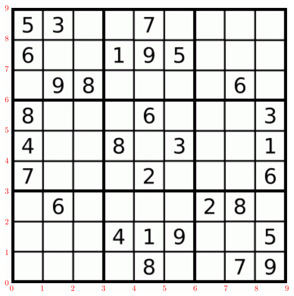
この場合は右下を (0,0)、左上を (9,9) としています。このようにすれば升目と座標が (ほぼ) 一致するので、かなりラクになると思います。後はさきほどと同様に、\node 等で必要な情報を入れていけば OK です。

さらなる深みへ

学術系の文書などでは上の方法で十分と思いますが、さらに以下のような変態ちっくなこともできます。えぇ TikZ ですから。

吹き出し

プレゼンなどでは吹き出しを使って注目してもらいたい点を強調したいかもしれません。その場合はその名の通りの shapes.callouts ライブラリーを使えばこんな感じにできます。ここでは基本パターンを挙げるだけにしておきます。他のバリエーション等については PGF マニュアルを参照して下さい (後の方の例でもいくつか使用しています)。

% duck-callout.tex
% \usetikzlibrary{shapes.callouts}

\begin{tikzpicture}
  \node[anchor=south west,inner sep=0] (duck) at (0,0) {%
    \includegraphics[width=0.75\textwidth]{640px-Duck0001.jpg}%
  };
  \begin{scope}[x={(duck.south east)},y={(duck.north west)}]
    % 補助
    \draw[help lines,xstep=.1,ystep=.1] (0,0) grid (1,1);
    \foreach \x in {0,1,...,9} { \node [anchor=north] at (\x/10,0) {0.\x}; }
    \foreach \y in {0,1,...,9} { \node [anchor=east]  at (0,\y/10) {0.\y}; }

    % 注釈
    \node[text=white, draw=white,  line width=1pt,
    ellipse callout,
    callout absolute pointer={(0.45, 0.6)}, % 吹き出しの開始位置
    ] at (0.3,0.5)     % 吹き出し本体の位置
    { \bf Wow! };
  \end{scope}
\end{tikzpicture} 

なお callouts パッケージというのもあります。やや柔軟性に乏しい感がありますが、あまりこだわりがなければこちらを使うのも手かもしれません。

% duck-callout-package.tex
% \usepackage[wby]{callouts}

\begin{annotate}{\includegraphics[width=0.75\textwidth]{640px-Duck0001.jpg}}{0.5}
  \helpgrid
  \callout{-5,-2}{\color{white}{\bf Wow!}}{-1,1.5}
\end{annotate}

一部拡大

あまり使い道が無いような気もしますが、こんなこともできます。いかにも TikZ な感じ (つまり変態) です。

% duck-spy.tex
% \usetikzlibrary{spy}

\begin{tikzpicture}[spy using outlines={circle, size=2.8cm, magnification=3, connect spies}]
  \node[anchor=south west,inner sep=0] (duck) at (0,0) {%
    \includegraphics[width=0.75\textwidth]{640px-Duck0001.jpg}%
  };
  \begin{scope}[x={(duck.south east)},y={(duck.north west)}]
    % 補助
    \draw[help lines,xstep=.1,ystep=.1] (0,0) grid (1,1);
    \foreach \x in {0,1,...,9} { \node [anchor=north] at (\x/10,0) {0.\x}; }
    \foreach \y in {0,1,...,9} { \node [anchor=east]  at (0,\y/10) {0.\y}; }
    % 注釈
    \node[text = red] at (0.45,0.35) { \tiny Wow! };

    % 拡大
    \node (target) at (0.45,0.35) {};    % 拡大箇所
    \node (mag)    at (0.18,0.72) {};    % 拡大図を置く位置
    \spy [white] on (target) in node at (mag);

    % 注意: 直接数字で座標を指定すると tikzpicture 側の座標系になる
    \spy [black, magnification=2, size=2cm, very thick] on (7,1) in node at (2,1.5);
  \end{scope}
\end{tikzpicture}

gnuplot との連携

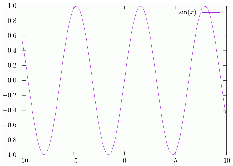
基本のおさらい

グラフを \LaTeX 文書に組み込む代表的は方法はおそらく gnuplot を使うことでしょう (gnuplot は極力最新版を使いましょう)。.tex ファイルの中から呼び出すこともできますが、ここでは (主に個人的な嗜好から) gnuplot 用のファイルを作成し、その中で .tex ファイルを生成し、それを \input する、という場合を想定します。なお、一昔前なら terminal^(*1) に eps 等を使用するというのもありましたが、今は tikz 一択です (断言)。

^(*1) 細かいことを言うと、terminal tikz は terminal lua tikz の略です。また、以下では terminal と書いていますが、term (つまり set term tikz) でも OK です。

まず、gnuplot ファイルを作成します。拡張子はあまり統一されていない気がしますが .gp とか .plt とかが多いでしょうか。私は .plot を使ってますが。その辺はお好きにどうぞ。

# sin.plot
set terminal tikz
set output "plot-sin.tex"

set format y "$%.1f$"

plot sin(x) title "$\\sin(x)$"

このファイルに対して gnuplot sin.plot を実行すると plot-sin.tex が生成されるので、それを \input すれば OK です。プリアンブルに \usepackage{gnuplot-lua-tikz} を入れるのを忘れないようにしましょう。

% sin.tex
% \usepackage{gnuplot-lua-tikz}
\input{plot-sin}

もちろん実際には figure 環境を使用すべきですが、ここでは省略しています。
また、私は混乱を避けるため生成されるファイルには plot- 等のプレフィックスを付けるようにしていますが、plot/ 等に生成するようにする、とか気にしない、とかでも良いでしょう。

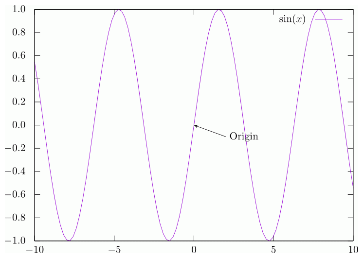
簡単な注釈

矢印と文字だけなら gnuplot の中でやってしまう方が楽かもしれません。

# sin-annotate.plot
set terminal tikz
set output "plot-sin-annotate.tex"

set format y "$%.1f$"

set arrow from 2,-0.1 to 0,0
set label at 2,-0.1 left " Origin"

plot sin(x) title "$\\sin(x)$"

% sin-annotate.tex
% \usepackage{gnuplot-lua-tikz}

\input{plot-sin-annotate}

一部拡大

上で紹介した spy ライブラリーでは「一部」を「そのまま」拡大してしまいますが、そうではなくて拡大用のグラフをさらに別途用意したい、ということも多いでしょう。この場合は gnuplot の multiplot 機能を使うのが一般的です。ここでは URL を紹介するにとどめておきます。”gnuplot inset” あたりでググるといろいろ出てきます。

• Mapt – Developer skills delivered
• 論文に使えるグラフをgnuplotで作る(応用編その3: インセットつきの図を作る)

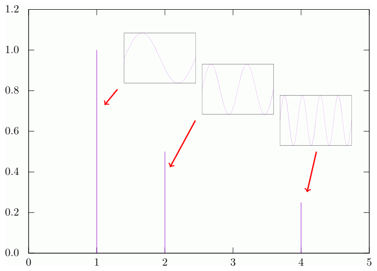
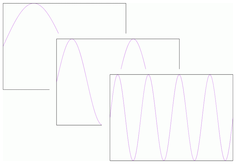
複数のグラフを重ねる

multiplot 的なことを TikZ で行うことも (一応) できます。

# fourier.plot
set terminal tikz
set output "plot-fourier.tex"

set format y "$%.1f$"

plot [0:5] [0:1.2] "-" using 1:2 with impulses notitle
1.0 1.0
2.0 0.5
4.0 0.25
end

# ------------------------------------------------------------
unset xlabel
unset ylabel
unset tics

do for [i=0:2] {
    set output "plot-sin" . i . ".tex"
    plot [0:2*pi] sin((2**i) * x) notitle
}

% fourier.tex
\begin{tikzpicture}
\node (overview) {\input{plot-fourier}};

\foreach \n in {0, 1, 2} {
  \node at (-1+2.5*\n, 2.5-\n) (sin\n) {\scalebox{0.2}{\input{plot-sin\n}}};
}

\draw[->, red, very thick] (sin0.south west) -- (-2.8, 1);
\draw[->, red, very thick] (sin1.south west) -- (-0.7,-1);
\draw[->, red, very thick] (sin2.south) -- ( 3.7,-1.8);
\end{tikzpicture}

% sins.tex
\begin{tikzpicture}
\foreach \i in { 0, 1, 2 } {
  \node[fill=white] at (3*\i, -2*\i) (sin\i) {\scalebox{0.6}{\input{plot-sin\i}}};
}
\end{tikzpicture}

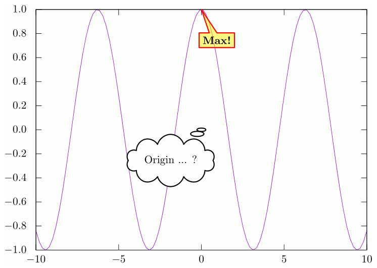
TikZ との連携

実はこれが本記事のメインです。この方法を見つけるのにかなりググったりしたのですが見つけられず、結局ソースを読んでようやく解決に至りました。という話はさておき、gnuplot で作成したグラフの中に TikZ で装飾したい、という場合、gnuplot 側で適切な箇所にアンカーを付けておくとさらに柔軟/簡潔に記述できます。このとき、若干のテクニック (?) が必要になります。と言っても、

1. terminal に nopicenvironment を指定する
2. set label "" at 0,0 font ",gp refnode,name=origin" のようにして node を作成する

くらいですが。簡単な例で見てみましょう。

# cos.plot
set terminal tikz nopicenvironment

set output "plot-cos.tex"
set format y "$%.1f$"

set label "" at 0,0 font ",gp refnode,name=origin"
set label "" at 0,1 font ",gp refnode,name=max"

plot cos(x) notitle

こんな感じになります。
このようにすると、生成される plot-cos.tex ファイル内の記述は、

\node[gp node left,font=,gp refnode,name=origin] at (6.572,4.529) {};

となるので、これを使って、

% cos.tex
% \usetikzlibrary{shapes.callouts}
% \usepackage{gnuplot-lua-tikz}

\begin{tikzpicture}[gnuplot]
  \input{plot-cos}

  \node[draw=red, line width=1pt, fill=yellow, fill opacity=0.5, text=black, text opacity=1,
  rectangle callout, callout absolute pointer={(max)}]
  at ($(0.5,-1)+(max)$) { \bf Max! };

  \node[draw, line width=1pt, fill=white,
  cloud callout, aspect=2.5, callout absolute pointer={(origin)}]
  at ($(-1,-1)+(origin)$) { Origin ... ? };
\end{tikzpicture}

とすればこんな図ができあがります。

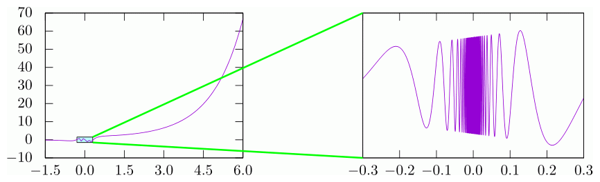
さらに、gnuplot で作成した複数の (独立した) .tex ファイルを並べてこれらの間で連携する、ということもできます。この場合、(少なくとも) 2回コンパイルが必要になります。

# esin.plot
set terminal tikz nopicenvironment scale 0.5,0.5

set output "plot-esin1.tex"

set xtics -1.5,1.5,6
set format x "$%.1f$"

set object 1 rectangle from -0.3,-1.5 to 0.3,1.5 fc rgb "#bb00ffff"
set label "" at 0.3, 1.5 font ",gp refnode,name=orig ne"
set label "" at 0.3,-1.5 font ",gp refnode,name=orig se"

plot [-1.5:6] exp(x)*sin(1/x) notitle

# ------------------------------------------------------------
reset

set output "plot-esin2.tex"

set noytics
set format x "$%.1f$"

set label "" at -0.3, 1.5 font ",gp refnode,name=enlarge nw"
set label "" at -0.3,-1.5 font ",gp refnode,name=enlarge sw"

set sample 20000
plot [-0.3:0.3] [-1.5:1.5] exp(x)*sin(1/x) notitle

% esin.tex
% \usepackage{gnuplot-lua-tikz}

% 2回コンパイルする必要あり
\begin{minipage}{0.5\linewidth}
  \begin{tikzpicture}[gnuplot, remember picture]
    \input{plot-esin1}     
  \end{tikzpicture}
\end{minipage}%
\begin{minipage}{0.5\linewidth}
  \begin{tikzpicture}[gnuplot, remember picture]
    \input{plot-esin2};   
  \end{tikzpicture}
\end{minipage}
\begin{tikzpicture}[remember picture, overlay]
  \draw[very thick, green] (orig ne) -- (enlarge nw);
  \draw[very thick, green] (orig se) -- (enlarge sw);
\end{tikzpicture}

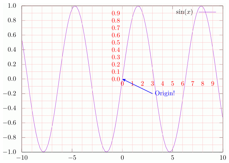
もし、グラフの座標系と同じ座標系を設定したければ、

# sin-grid.plot
set terminal tikz nopicenvironment

set output "plot-sin-grid.tex"
set format y "$%.1f$"

set label "" at 0,0 font ",gp refnode,name=orig"
set label "" at 1,0 font ",gp refnode,name=x1"
set label "" at 0,1 font ",gp refnode,name=y1"

plot sin(x) title "$\\sin(x)$"

% sin-grid.tex
% \usepackage{gnuplot-lua-tikz}

\begin{tikzpicture}[gnuplot]
  \input{plot-sin-grid}

  \begin{scope}[shift={(orig)},x={(x1)},y={(y1)}]
    % 補助
    \draw[draw=pink,xstep=1,ystep=0.1] (-10,-1) grid (10,1);
    \foreach \x in {0,1,...,9} { \node [red, anchor=north] at (\x,0) {\x}; }
    \foreach \y in {0,1,...,9} { \node [red, anchor=east]  at (0,\y/10) {0.\y}; }

    % 注釈
    \draw[<-, thick, blue] (0,0) -- (3,-0.2);
    \node[anchor=west, blue] at (3,-0.2) { Origin! };
  \end{scope}
\end{tikzpicture}

のようにすることもできます。つまり、.plot ファイル内で主要な点 (ここでは原点, (1,0), (0,1)) に名前を付けておいて、.tex 内でそれらを使って座標系を定義します。

もちろん (?) 三次元でも OK です。

# 3D.plot
set terminal tikz nopicenvironment
set output "plot-3D.tex"

unset hidden3d

set samples 21
set isosample 11

set label "" at 0,0,0 font ",gp refnode,name=origin"

# これだと誤差が大きくてズレてしまう
# set label "" at 1,0,0 font ",gp refnode,name=xx"
# set label "" at 0,1,0 font ",gp refnode,name=yy"
# set label "" at 0,0,1 font ",gp refnode,name=zz"

set label "" at 10,0,0  font ",gp refnode,name=x10"
set label "" at 0,10,0  font ",gp refnode,name=y10"
set label "" at 0,0,100 font ",gp refnode,name=z100"

splot [-10:10] [-10:10] x*y notitle

% 3D.tex
% \usetikzlibrary{calc}
% \usepackage{gnuplot-lua-tikz}

\begin{tikzpicture}[gnuplot]
  \input{plot-3D}

  \begin{scope}[shift={(origin)},x={($0.1*(x10)$)},y={($0.1*(y10)$)},z={($0.01*(z100)$)}]
    \draw[<-, thick, red]  (-10,-10,100) -- (10,-10,-100);
    \draw[->, thick, blue] (10,-10,-100) -- (10,10,100);

    \node[draw, line width=1pt, fill=white,
    ellipse callout, callout absolute pointer={(origin)}]
    at ($(0,0,50)+(origin)$) { Origin };
  \end{scope}
\end{tikzpicture}

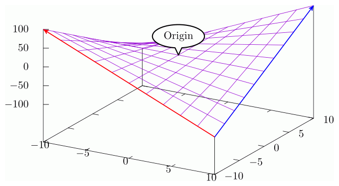
図の中に TikZ で赤と青の矢印を描いてみましたが、この例の場合だと (1,0,0) 等を使用して座標系を定義すると誤差が発生し線がズレてしまいます (3D.plot 内のコメント参照)。ので (10,0,0) などを使用し、これを長さで割ることで、ズレを抑えています。

\begin{scope}[shift={(orig)},x={(x1)},y={(y1)}]

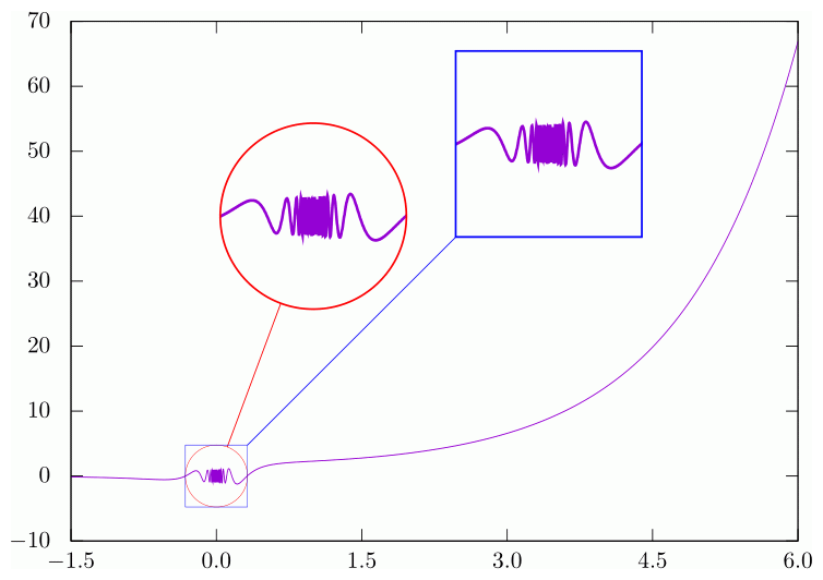
なお、当然 spy を使うこともできますが、すでに述べたように spy は単純に拡大するだけなので、場合によっては期待通りにはなりません。次の例では(ほぼ)「期待通り」にするために .plot ファイル内で set sample を使って描画点の数を増やしています (実は上でもすでに使用しています)。ただし、ファイルサイズやコンパイル時間が無駄に大きくなる^(*2) ので、あまりおすすめしません (もちろん本当に必要なら使用すべきですが)。

^(*2) 今回は述べませんが、必要に応じて tikzexternalize を使うと良いでしょう。

# esin-spy.plot
set terminal tikz nopicenvironment

set output "plot-esin-spy.tex"

set format x "$%.1f$"
set xtics -1.5,1.5,6

set label "" at 0.0, 0.0 font ",gp refnode,name=target"
set label "" at 1.0,40.0 font ",gp refnode,name=mag"

set sample 10000

plot [-1.5:6] exp(x)*sin(1/x) notitle

% esin-spy.tex
% \usetikzlibrary{spy}
% \usepackage{gnuplot-lua-tikz}

\begin{tikzpicture}[gnuplot, spy using outlines={circle, size=2.8cm, magnification=3, connect spies}]
  \input{plot-esin-spy}

  % 共にアンカーを使う場合
  \spy [red]  on (target) in node at (mag);

  % TikZ 側の座標を併用する場合
  \spy [blue, rectangle] on (target) in node at ($(target)+(5,5)$);
\end{tikzpicture}

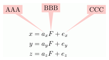
おまけ: 数式中に callout でコメントを入れる

図ではありませんが、かなり関連した情報なので紹介しておきます。
元ネタはこちら: TeX Forum

% eq-callouts.tex
% \usepackage{amsmath}
% \usetikzlibrary{positioning}
% \usetikzlibrary{shapes.callouts}

\begin{align}
  x & = \tikz[remember picture,baseline=(fs.base),outer sep=0pt,inner sep=0pt]{\node(fs){$a_x$};}%
     \tikz[remember picture,baseline=(cs.base),outer sep=0pt,inner sep=0pt]{\node(cs){$F$};}+%
     \tikz[remember picture,baseline=(sf.base),outer sep=0pt,inner sep=0pt]{\node(sf){$e_x$};} \\
  y & = a_yF+e_y \\
  z & = a_zF+e_z
\end{align}

\begin{tikzpicture}[remember picture,overlay,
  every node/.style={rectangle callout,fill=red!20,overlay}]
  \node[callout absolute pointer=(fs.north),above left=of fs]{AAA};
  \node[callout absolute pointer=(cs.north),above=of cs]{BBB};
  \node[callout absolute pointer=(sf.north),above right=of sf]{CCC};
\end{tikzpicture}

いらないあとがき

ということで、もしかすると論文作成やプレゼンテーション等で使えるかもしれない技を紹介しました。よろしければ twitter あたりで感想や改善案等をいただけると幸いです。

本記事は TikZ を扱っている割には、それほど変態的ではなかったかもしれません。

ちなみに今回がアレカレンダー初参加です。書くからにはきちんとした記事を書かないと、と気負いすぎた感があります。詰め込みすぎて理解しにくくなっていないと良いのですが。

では、ちょっと早いですが良いクリスマスを。

References:

本文中でリンクしたものは除きます。

• なにはなくとも TikZ & PGF Manual
• gnuplot
• 画像取り込み, 座標系指定, グリッドについては、困った時の Stack Exchange
• アヒルの写真は Wikimedia より
• 数独の図も Wikimedia より
• spy ライブラリについては rinx’s memo を参考にさせていただきました (2019年12月現在、404。Internet Archive)